JHU Plots
wide_us_cases <- us_state %>% select(- deaths) %>%
  pivot_wider(names_from = state, values_from = cases) %>%
  tk_xts(., date_var = date)

wide_us_deaths <- us_state %>% select(- cases) %>%
  pivot_wider(names_from = state, values_from = deaths) %>%
  tk_xts(., date_var = date)
wide_china_cases <- china_state %>%
select(- deaths, - recovered, - active) %>%
pivot_wider(names_from = state, values_from = cases) %>%
tk_xts(., date_var = date)
wide_china_deaths <- china_state %>%
select(- cases, - recovered, - active) %>%
pivot_wider(names_from = state, values_from = deaths) %>%
tk_xts(., date_var = date)
wide_china_recovered <- china_state %>%
select(- deaths, - cases, - active) %>%
pivot_wider(names_from = state, values_from = recovered) %>%
tk_xts(., date_var = date)
wide_china_active <- china_state %>%
select(- cases, - recovered, - deaths) %>%
pivot_wider(names_from = state, values_from = active) %>%
tk_xts(., date_var = date)wide_world_cases <- world %>%
select(- deaths, - recovered, - active) %>%
pivot_wider(names_from = country, values_from = cases) %>%
tk_xts(., date_var = date)
wide_world_deaths <- world %>%
select(- cases, - recovered, - active) %>%
pivot_wider(names_from = country, values_from = deaths) %>%
tk_xts(., date_var = date)
wide_world_recovered <- world %>%
select(- deaths, - cases, - active) %>%
pivot_wider(names_from = country, values_from = recovered) %>%
tk_xts(., date_var = date)
wide_world_active <- world %>%
select(- cases, - recovered, - deaths) %>%
pivot_wider(names_from = country, values_from = active) %>%
tk_xts(., date_var = date)USA
ggplots
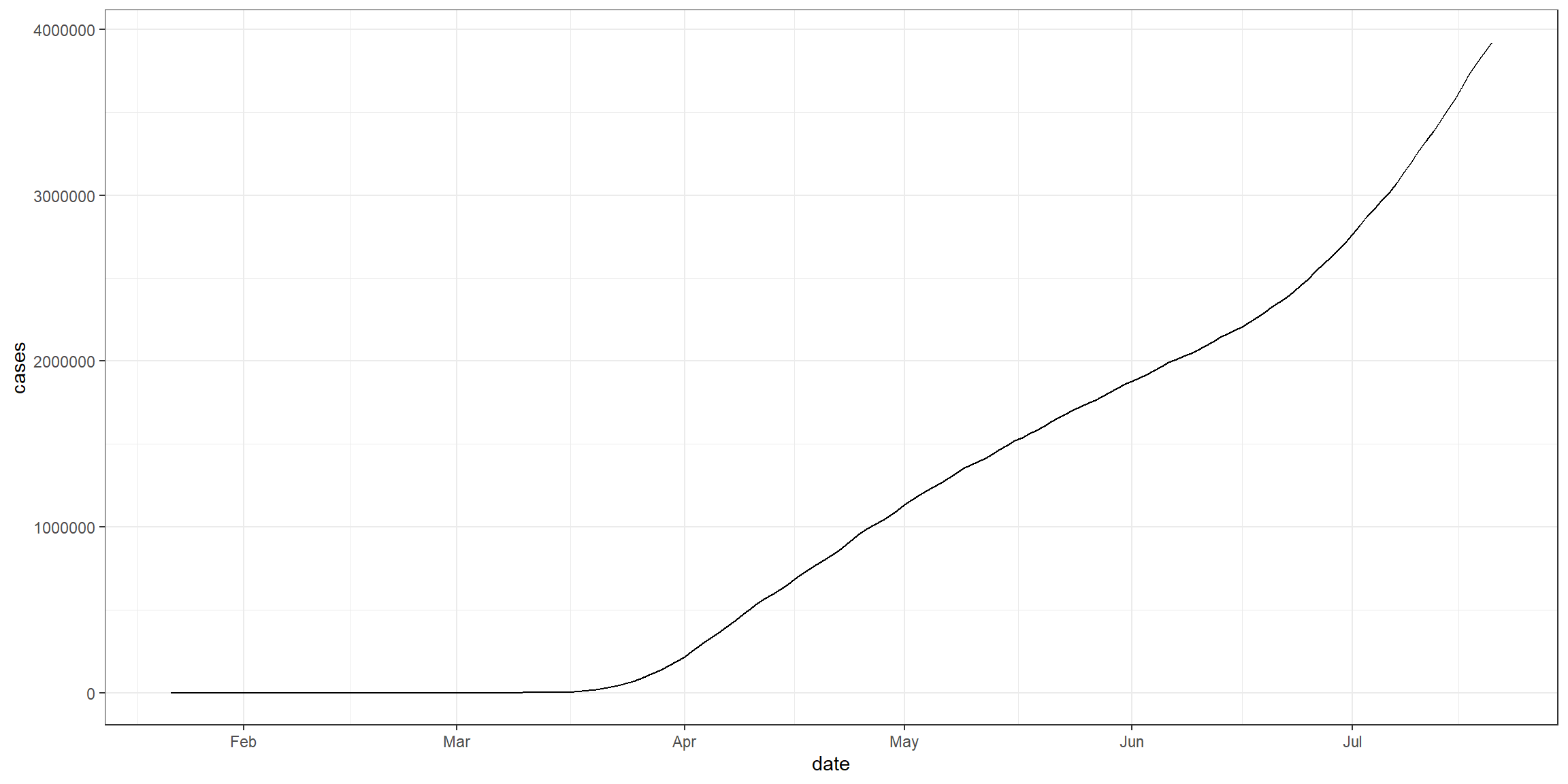
This is a basic graph of USA’s cases of COVID-19 by date.
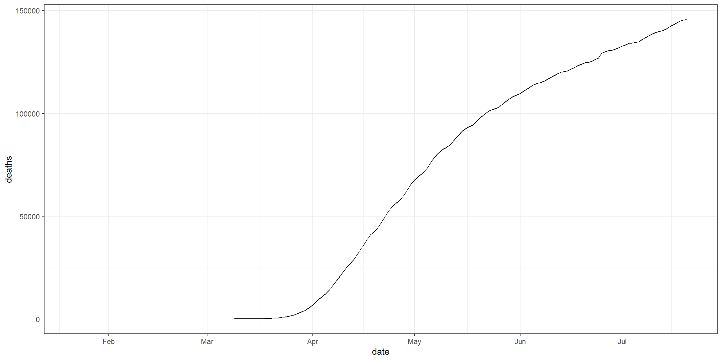
This is a basic graph of USA’s deaths of COVID-19 by date.
dygraphs
dygraph(wide_us_cases) %>%
  dyRangeSelector(height = 20, strokeColor = "") %>%
  dyAxis("y", label = "cases")
This is an interactive graph of USA’s cases of COVID-19 by date.
dygraph(wide_us_deaths) %>%
  dyRangeSelector(height = 20, strokeColor = "") %>%
  dyAxis("y", label = "deaths")
This is an interactive graph of USA’s deaths of COVID-19 by date.
China
ggplots
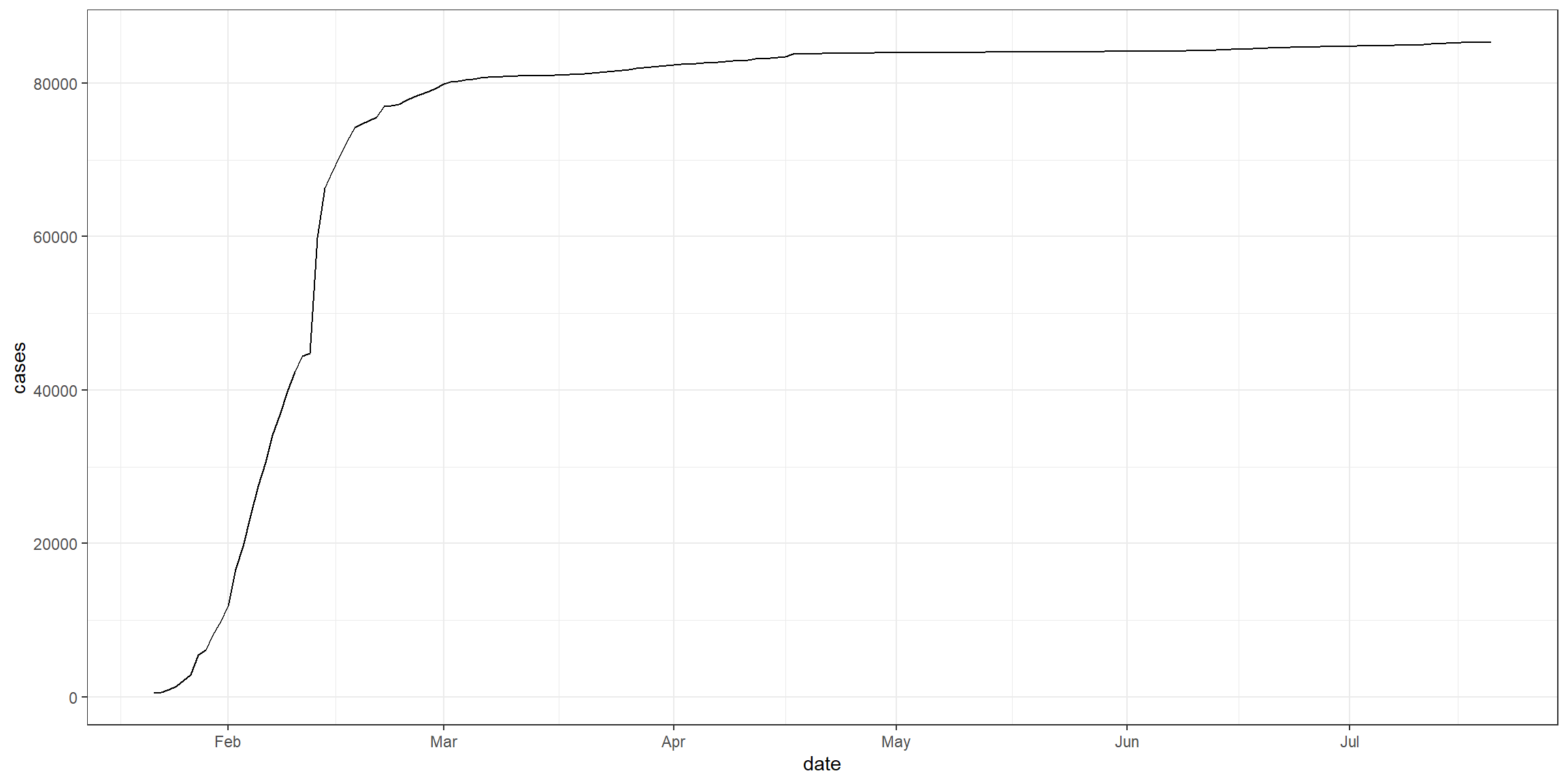
This is a basic graph of China’s cases of COVID-19 by date.
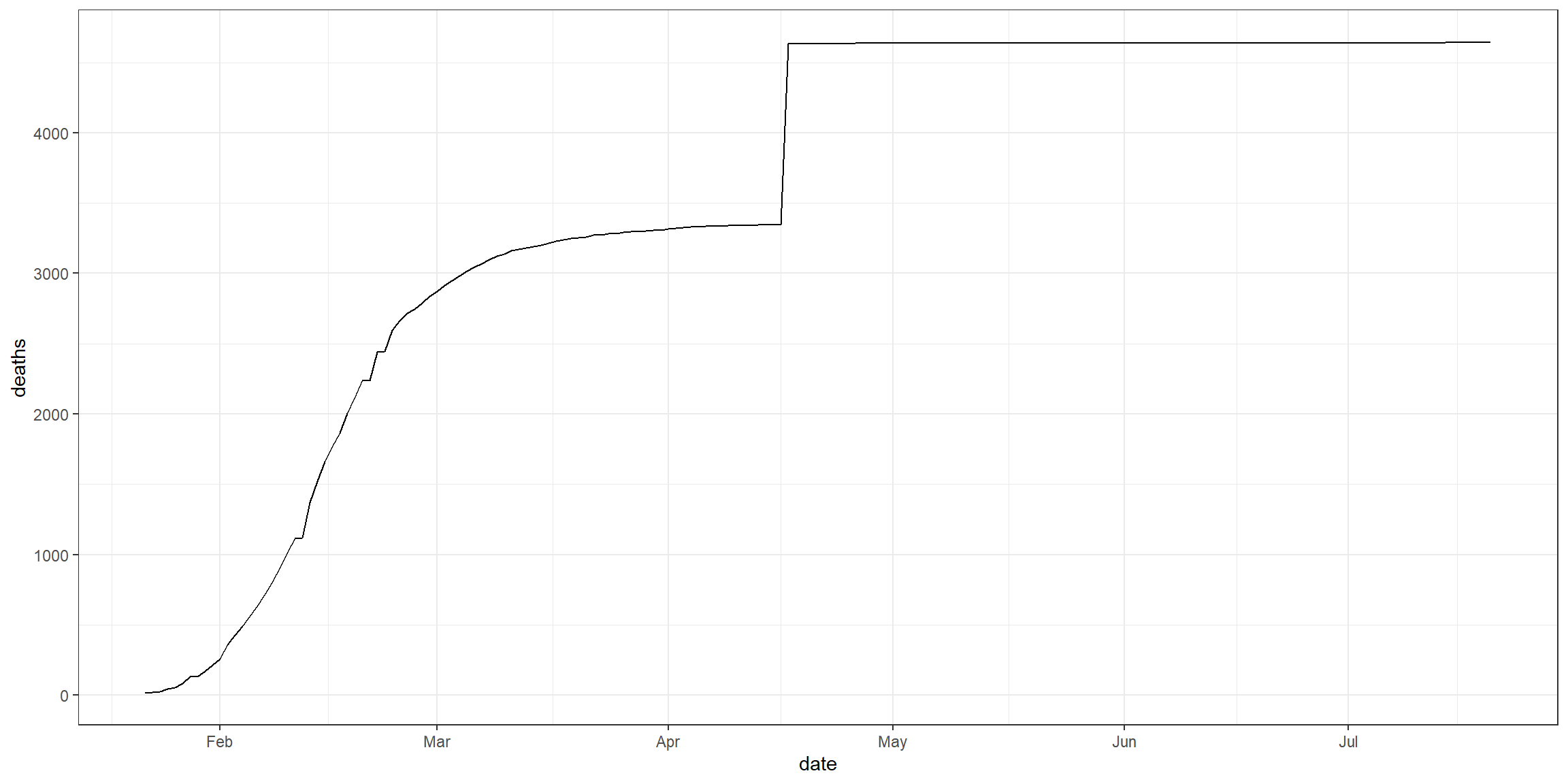
This is a basic graph of China’s deaths of COVID-19 by date.
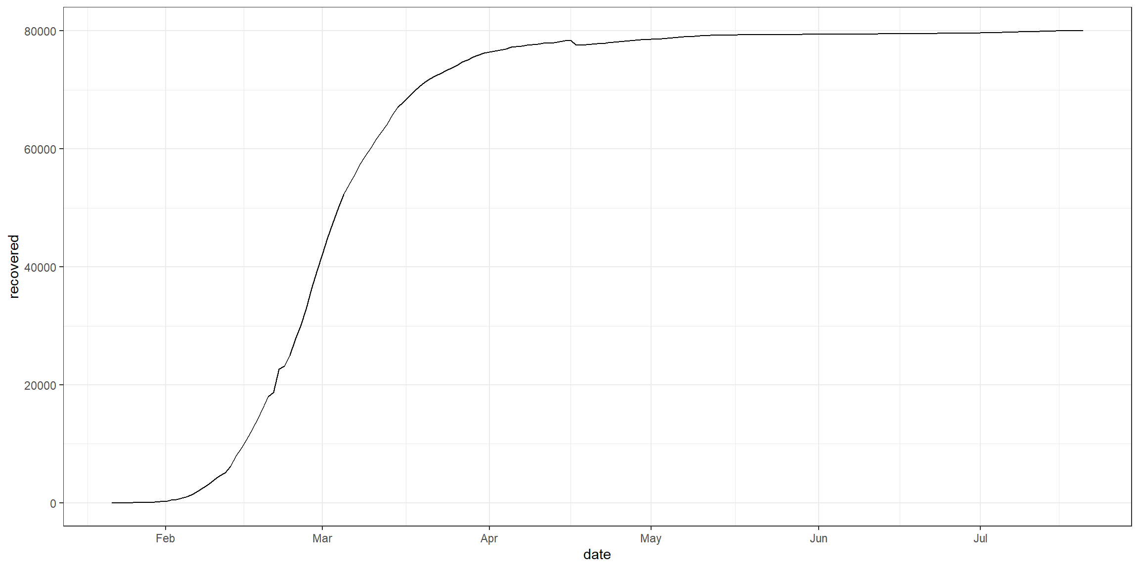
This is a basic graph of China’s recovered patients of COVID-19 by date.
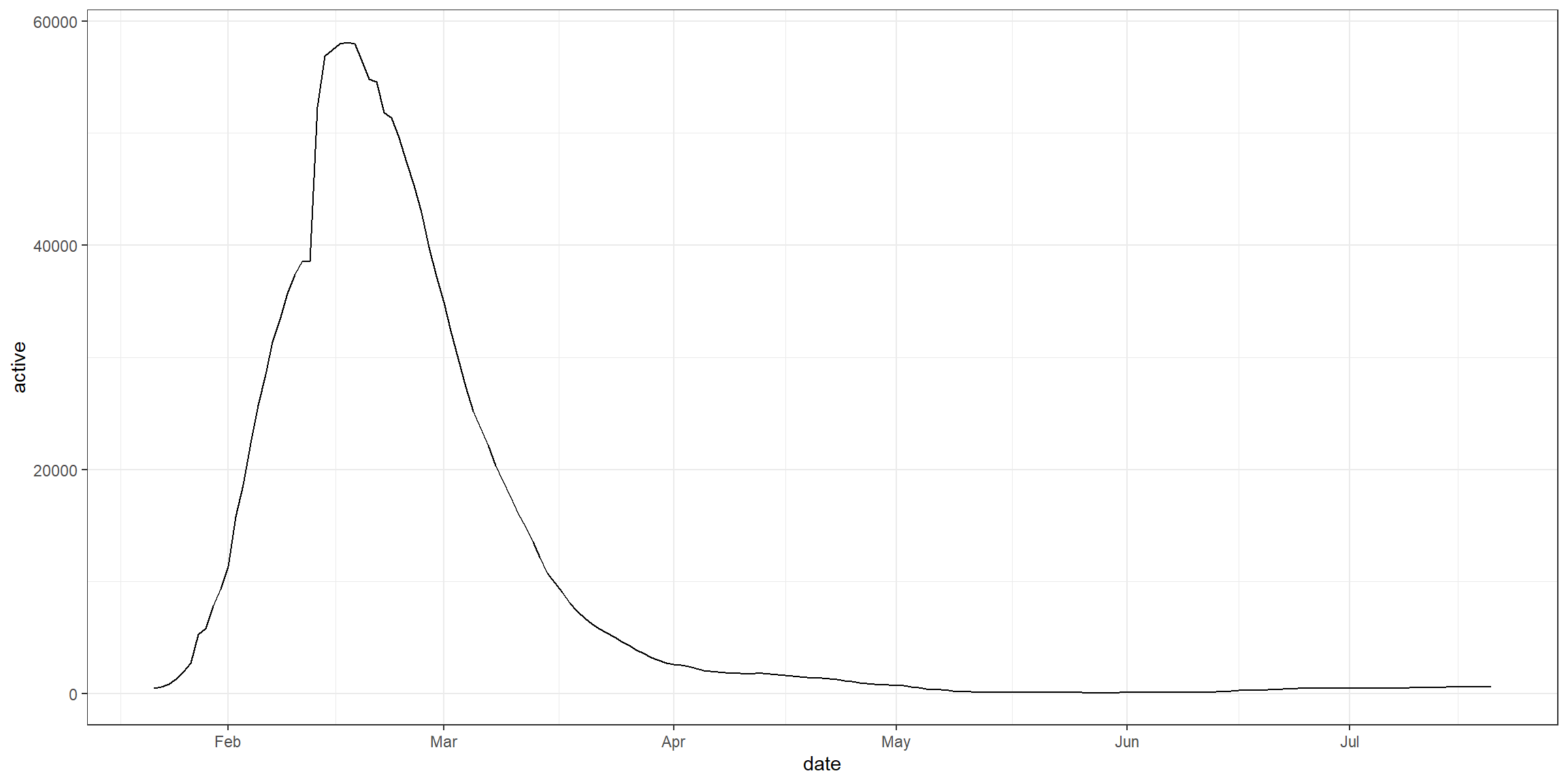
This is a basic graph of China’s active cases of COVID-19 by date.
dygraphs
dygraph(wide_china_cases) %>%
  dyRangeSelector(height = 20, strokeColor = "") %>%
  dyAxis("y", label = "cases")
This is an interactive graph of China’s cases of COVID-19 by date.
dygraph(wide_china_deaths) %>%
  dyRangeSelector(height = 20, strokeColor = "") %>%
  dyAxis("y", label = "deaths")
This is an interactive graph of China’s deaths of COVID-19 by date.
dygraph(wide_china_recovered) %>%
  dyRangeSelector(height = 20, strokeColor = "") %>%
  dyAxis("y", label = "recovered")
This is an interactive graph of China’s recovered patients of COVID-19 by date.
dygraph(wide_china_active) %>%
  dyRangeSelector(height = 20, strokeColor = "") %>%
  dyAxis("y", label = "active")
This is an interactive graph of China’s active cases of COVID-19 by date.
World
The countries plotted are Australia, China, Denmark, France, Netherlands, and United Kingdom.
ggplots
ggplot(data = world, aes(x = date, y = cases, fill = country)) +
  geom_col() + facet_wrap(~country) +
  theme_bw()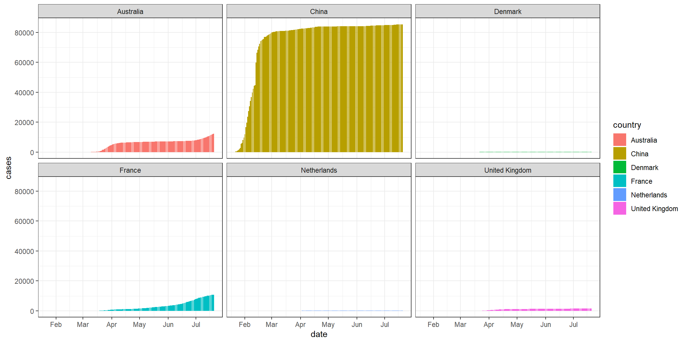
This is a basic graph of multiple countries’ cases of COVID-19 by date.
ggplot(data = world, aes(x = date, y = deaths, fill = country)) +
  geom_col() + facet_wrap(~country) +
  theme_bw()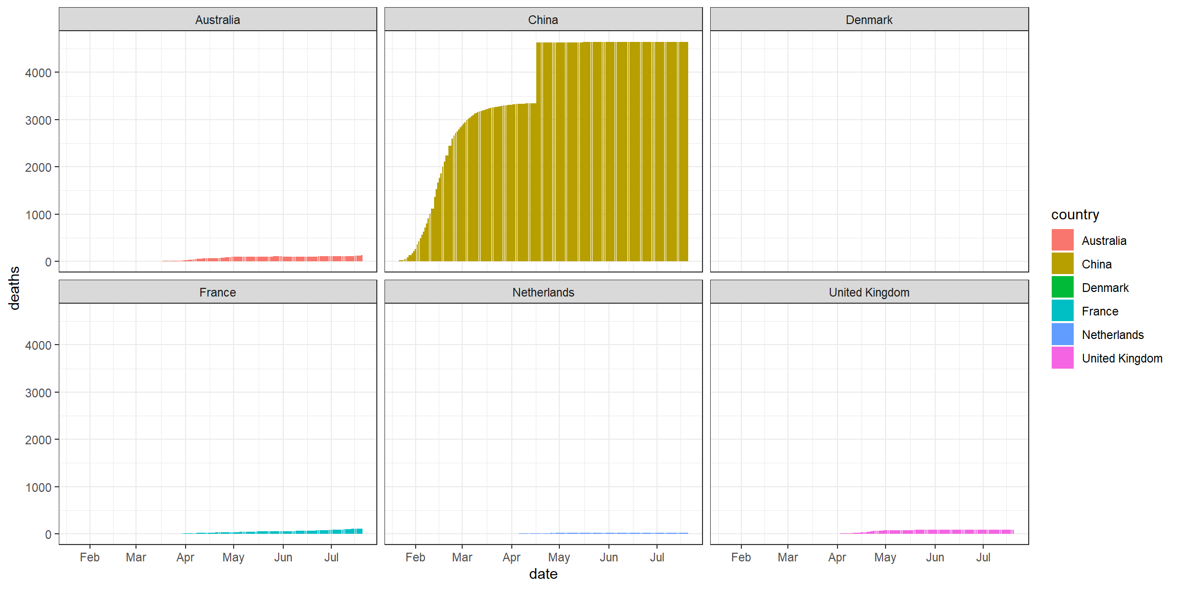
This is a basic graph of multiple countries’ deaths of COVID-19 by date.
ggplot(data = world, aes(x = date, y = recovered, fill = country)) +
  geom_col() + facet_wrap(~country) +
  theme_bw()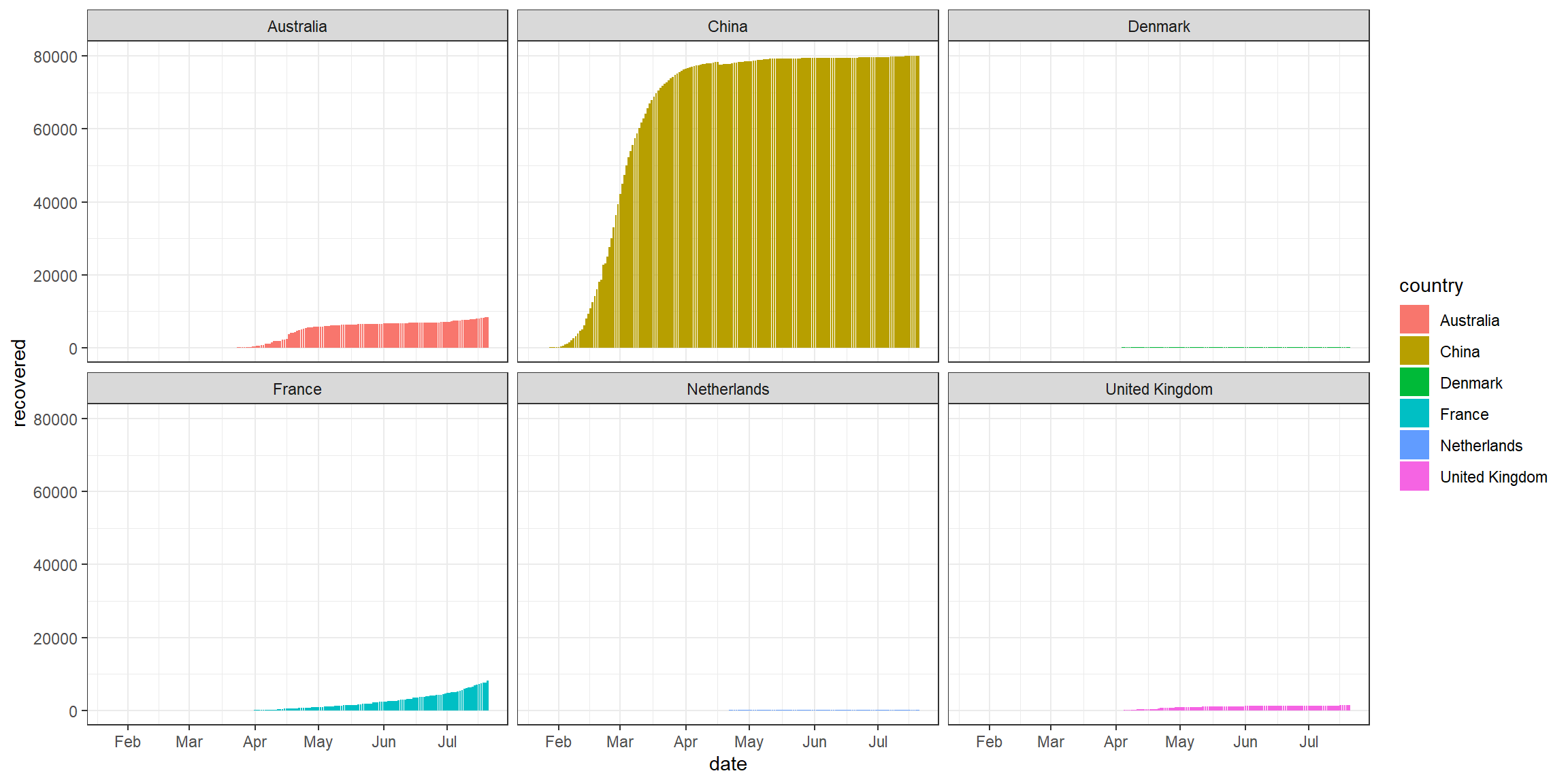
This is a basic graph of multiple countries’ recovered patients of COVID-19 by date.
ggplot(data = world, aes(x = date, y = active, fill = country)) +
  geom_col() + facet_wrap(~country) +
  theme_bw()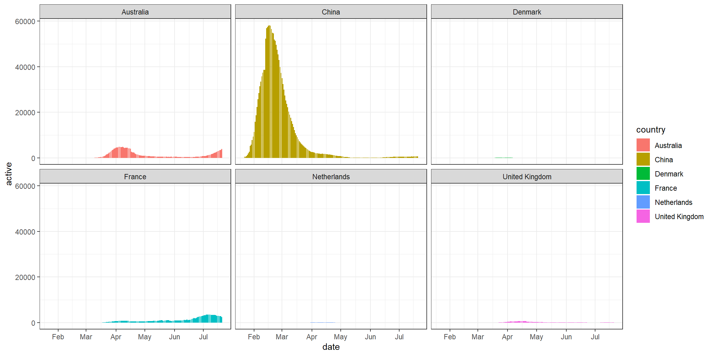
This is a basic graph of multiple countries’ active cases of COVID-19 by date.
dygraphs
dygraph(wide_world_cases) %>%
  dyRangeSelector(height = 20, strokeColor = "") %>%
  dyAxis("y", label = "cases")
This is an interactive graph of multiple countries’ cases of COVID-19 by date.
dygraph(wide_world_deaths) %>%
  dyRangeSelector(height = 20, strokeColor = "") %>%
  dyAxis("y", label = "deaths")
This is an interactive graph of multiple countries’ deaths of COVID-19 by date.
dygraph(wide_world_recovered) %>%
  dyRangeSelector(height = 20, strokeColor = "") %>%
  dyAxis("y", label = "recovered")
This is an interactive graph of multiple countries’ recovered patients of COVID-19 by date.
dygraph(wide_world_active) %>%
  dyRangeSelector(height = 20, strokeColor = "") %>%
  dyAxis("y", label = "active")
This is an interactive graph of multiple countries’ active cases of COVID-19 by date.
## [1] "Last updated: Jul 21 2020"